How to build a neural network for MNIST using tensorflow

Instroduction

The first step to dive into machine learning is to do experiment on MNIST dataset for most of beginers. MNIST is a dataset of handwriting digits. Beginners can learn fundamental knowledge from creating program to recognize digits, while researchers can develope new algorithmns and models upon it. It is said that it’s no guarantee that one algorithmn working well on MNIST works well on the other domain, but it’s guaranteed that one algorithmn doesn’t work well on the domain if it does’nt work well on MNIST.

In my case, I’m a beginer of machine learning, furthermore digit recognition is one of my production challenge. The problem is about recognizing non-embossed font digits on cards. The cards are fixed size with various background, pure color or images. The digits are arranged in 4x4 grid with fixed font size. However, as we can see, the digit size can not be guaranteed due to two obvious reasons. One is caused by the font itselft. Each digit from 0 to 9 doesn’t occupy the same area on the card. The another is caused by the distance of the card and the camera.

Anyway, the first step is to try MNIST since there is no enough images to develop digit recongnition model. By try MNIST, I can learn the fundamental knowledge of develop a model for digit recognition.

Articles

Before I dive into a thick book, I find some articles by googling to get a quick started.

• How to build a neural network to recognize handwritten digits with tensorflow
• Not another MNIST tutorial with tensorflow
• Visualizing MNIST

The first two lead me to understand how a linear classifier works and how to make such a classifier. The last one tells technologies for dimentional data reduction.

So, what are they?

Regression and Classification

Before we can apply any machine learning algorithmn, it’s critical to tell what kind of task we are going to do first, regression or classification. Both regression and classification tasks are predictive modeling problem. A predictive modeling is a problem of approximating a mapping function from input to output using historical data to predicate upon new data where we don’t have answer.

Classification predictive modeling is the task of approximating a mapping function (f) from input variables (X) to discrete output variables (y).

Regression predictive modeling is the task of approximating a mapping function (f) from input variables (X) to a continuous output variable (y).

More details can be found at Classification vs. Regression in machine learning.

Digit recognition is a classification problem that we’d want to give a label to a given image of a digit. In digit recognition case, image each label is a point in a 10-dimension space, and the whole space is separated by 10 lines. So the problem is modeled as the given image is transformed to a point in the space and the nearest line representing the label that the image should has. Then the problem becomes,

1. how to map the image to the point?
2. What is the line?
3. how to measure the distance?

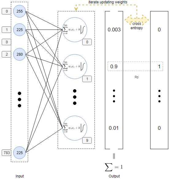
When we talk about label representation, it’s natrual to encode the 10 labels into a vector in which the value of the position representing the label is 1, and others are 0. For example, for a image of digit 3, the vector is [0,0,0,1,0,0,0,0,0,0]. This vector can also be interpreted as the 1 means the probability of that the image belongs to the cooresponding label is 100%. Because a image can belong to one category in the case, so the probabilities of others are of cause 0. If the vector is the combination of probabilities of that the image belongs to each category, the line of these points is a kind of probability distribution. All images with the same label should be on the line or near to it. Since we are measuring distance of probability distribution, cross-entropy is one of good choice.

Till now, the classification problem is transformed into a linear regression problem. The model function is y = Wx + b modeling a line and cross-entropy is used to optimize W so that for a given example, the best y is predicted.

Single Layer Neural Network

Not another MNIST tutorial with tensorflow gives a single layer Neural Network for this problem. An image of 28x28 is flat as a 1x784 vector to be the input layer of the network. Each pixel of the image is a node in the network linking to neuron in the output layer. As discussed previously, there are 10 neuron in the output layer to give a 1x10 vector as output in which each number in a position representing the probability of that the image belongs to that category. Each neuron accepts 784 inputs and give one output. The output is the input multiplying Weight and adding a Bias.

$$y = \begin{bmatrix}w_{0,0} & w_{0,1} & w_{0,2} & \cdot & \cdot & \cdot & w_{0,783}\\w_{1,0} & \cdot & \cdot & \cdot & & & w_{1,783} \\ \cdot & & & & & & \\ \cdot & & & & & & \\ \cdot & & & & & & \\ w_{9, 0} & w_{9,1} & \cdot & \cdot & \cdot & & w_{9,783} \end{bmatrix} \times \begin{bmatrix}x_{0} \\ x_{1} \\ x_{2} \\ \cdot \\ \cdot \\ \cdot \\ x_{783} \end{bmatrix} + \begin{bmatrix}b_{0,0}\\b_{1,0}\\b_{2,0}\\ \cdot \\ \cdot \\ \cdot \\ b_{9,0} \end{bmatrix}$$

Architecture

The second article introduces a network of the following architecture. It’a a single layer neural network. There are 10 neuron in the layer because we want a 1x10 vector as output which is the one-hot encoding of the labels of the digits.

Step 1 Preparation

install dependencies

Execute the following commands to setup virtual environment for the project.

$ mkdir tensorflow-demo
$ cd tensorflow-demo
$ python3 -m venv tensorflow-demo
$ source tensorflow-demo/bin/activate

Next, install required libraries from requirements.txt.

$ touch requirements.txt

Add the following lines to the file.

image==1.5.20
numpy==1.14.3
tensorflow-gpu>=1.4.1
jupyter>=4.0

Save and install libraries by the following command.

$ pip install -r requirements.txt

With the dependencies installed, we can start with the project.

Use jupyter notebook remotely

Execute the following commands in Ubuntu to start up jupyter note book. The proxy is optional depending on the running environment.

$ export http_proxy=http://192.168.0.105:37103
$ export https_proxy=http://192.168.0.105:37103
$ jupyter notebook --no-browser
...
[C 16:32:11.532 NotebookApp]

    To access the notebook, open this file in a browser:
        file:///run/user/1000/jupyter/nbserver-6144-open.html
    Or copy and paste one of these URLs:
        http://localhost:8888/?token=f244ddc108cc3d1e33c4d868ba7c088b45bdd73a67a1bcf7

If we want to access the notebook from Windows, we need forward port by ssh. Open a cmder console to execute.

ssh -L 8080:localhost:8888 linwumeng@192.168.0.105

Then, we can open Chrome with url http://localhost:8080/?token=f244ddc108cc3d1e33c4d868ba7c088b45bdd73a67a1bcf7 to create a new notebook file.

Step 2 load images

An digital image is a real-value matrix as well. In our neural network, we expand 28x28 images into 1x784 vector as input by concatenating 28 rows into one.

from tensorflow.examples.tutorials.mnist import input_data
mnist = input_data.read_data_sets("MNIST_data/", one_hot=True)

Setting one_hot to be True means use a 1x10 vector to represent labels.

$$\begin{matrix}digit & label \\0 & \begin{bmatrix}{\color{Red} 1} & 0 & 0 & 0 & 0 & 0 & 0 & 0 & 0 & 0 \end{bmatrix}\\ 1 & \begin{bmatrix}0 & {\color{Red} 1} & 0 & 0 & 0 & 0 & 0 & 0 & 0 & 0 \end{bmatrix}\\ 2 & \begin{bmatrix}0 & 0 & {\color{Red} 1} & 0 & 0 & 0 & 0 & 0 & 0 & 0 \end{bmatrix}\\ 3 & \begin{bmatrix}0 & 0 & 0 & {\color{Red} 1} & 0 & 0 & 0 & 0 & 0 & 0 \end{bmatrix}\\ 4 & \begin{bmatrix}0 & 0 & 0 & 0 & {\color{Red} 1} & 0 & 0 & 0 & 0 & 0 \end{bmatrix}\\ 5 & \begin{bmatrix}0 & 0 & 0 & 0 & 0 & {\color{Red} 1} & 0 & 0 & 0 & 0 \end{bmatrix}\\ 6 & \begin{bmatrix}0 & 0 & 0 & 0 & 0 & 0 & {\color{Red} 1} & 0 & 0 & 0 \end{bmatrix}\\ 7 & \begin{bmatrix}0 & 0 & 0 & 0 & 0 & 0 & 0 & {\color{Red} 1} & 0 & 0 \end{bmatrix}\\ 8 & \begin{bmatrix}0 & 0 & 0 & 0 & 0 & 0 & 0 & 0 & {\color{Red} 1} & 0 \end{bmatrix}\\ 9 & \begin{bmatrix}0 & 0 & 0 & 0 & 0 & 0 & 0 & 0 & 0 & {\color{Red} 1} \end{bmatrix} \end{matrix}$$

The python code will download MNIST data from internet and unzip it into the folder MNIST_data under the path where we run jupyter notebook.

Next, we’d like to have a look at the data set. How many are there? What do they look like?

n_train = mnist.train.num_examples
n_test = mnist.test.num_examples

def TRAIN_SIZE(num):
    print ('Total Training Images in Dataset = ' + str(mnist.train.images.shape))
    print ('--------------------------------------------------')
    x_train = mnist.train.images[:num,:]
    print ('x_train Examples Loaded = ' + str(x_train.shape))
    y_train = mnist.train.labels[:num,:]
    print ('y_train Examples Loaded = ' + str(y_train.shape))
    print('')
    return x_train, y_train

def TEST_SIZE(num):
    print ('Total Test Examples in Dataset = ' + str(mnist.test.images.shape))
    print ('--------------------------------------------------')
    x_test = mnist.test.images[:num,:]
    print ('x_test Examples Loaded = ' + str(x_test.shape))
    y_test = mnist.test.labels[:num,:]
    print ('y_test Examples Loaded = ' + str(y_test.shape))
    return x_test, y_test

x_train, y_train = TRAIN_SIZE(n_train)
x_test, y_test = TEST_SIZE(n_test)

We will get the output,

Total Training Images in Dataset = (55000, 784)
--------------------------------------------------
x_train Examples Loaded = (55000, 784)
y_train Examples Loaded = (55000, 10)

Total Test Examples in Dataset = (10000, 784)
--------------------------------------------------
x_test Examples Loaded = (10000, 784)
y_test Examples Loaded = (10000, 10)

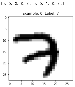
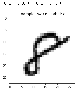
Let us have a look at same images in train set.

def display_digit(num):
    print(y_train[num])
    label = y_train[num].argmax(axis=0)
    image = x_train[num].reshape([28,28])
    plt.title('Example: %d  Label: %d' % (num, label))
    plt.imshow(image, cmap=plt.get_cmap('gray_r'))
    plt.show()

display_digit(0)
display_digit(54999)

Now, we have loaded MNIST dataset into the memory.

Step 3 Building the TensorFlow Graph

The architecture of the neural network refers to elements such as the number of layers in the network, the number of units in each layer, and how the units are connected between layers.

The term hidden layer is used for all of the layers in between the input and output layers, i.e. those “hidden” from the real world.

Our first neural network has only one layer of neurons as the output layer. The input layer accepts 784 pixels of the 28x28 image, then passing them to the output layer for computing. The output from the output layer is a 1x10 vector representing the predicted probability distribution of the images being of the categories which is used to compute cross entroy with the real distribution where only one position has value 1, and others are all 0.

n_input = 784 # input layer (28x28 pixels)
n_output = 10 # output layer (0-9 digits)

X = tf.placeholder(tf.float32, shape=[None, n_input])
Y = tf.placeholder(tf.float32, shape=[None, n_output])

W = tf.Variable(tf.zeros([n_input,n_output]))
b = tf.Variable(tf.zeros([n_output]))

y = tf.nn.softmax(tf.matmul(x,W) + b)

LEARNING_RATE = 0.1
TRAIN_STEPS = 10000
cross_entropy = tf.reduce_mean(-tf.reduce_sum(y_ * tf.log(y), reduction_indices=[1]))
training = tf.train.GradientDescentOptimizer(LEARNING_RATE).minimize(cross_entropy)

Step 4 Training and Testing

The training process involves feeding the training dataset through the graph and optimizing the loss function. Every time the network iterates through a batch of more training images, it updates the parameters to reduce the loss in order to more accurately predict the digits shown.

The testing process involves running our testing dataset through the trained graph, and keeping track of the number of images that are correctly predicted, so that we can calculate the accuracy.

correct_prediction = tf.equal(tf.argmax(y,1), tf.argmax(y_,1))
accuracy = tf.reduce_mean(tf.cast(correct_prediction, tf.float32))

init = tf.global_variables_initializer()
sess.run(init)

for i in range(TRAIN_STEPS+1):
    sess.run(training, feed_dict={x: x_train, y_: y_train})
    if i%500 == 0:
        print('Training Step:' + str(i) + '  Accuracy =  ' + str(sess.run(accuracy, feed_dict={x: x_test, y_: y_test})) + '  Loss = ' + str(sess.run(cross_entropy, {x: x_train, y_: y_train})))

Then, we get the output below,

Total Training Images in Dataset = (55000, 784)
--------------------------------------------------
x_train Examples Loaded = (5500, 784)
y_train Examples Loaded = (5500, 10)

Total Test Examples in Dataset = (10000, 784)
--------------------------------------------------
x_test Examples Loaded = (10000, 784)
y_test Examples Loaded = (10000, 10)
Training Step:0  Accuracy =  0.5988  Loss = 2.1881988
Training Step:500  Accuracy =  0.8943  Loss = 0.35697538
Training Step:1000  Accuracy =  0.9009  Loss = 0.3010645
Training Step:1500  Accuracy =  0.9048  Loss = 0.27260992
Training Step:2000  Accuracy =  0.9066  Loss = 0.2535662
Training Step:2500  Accuracy =  0.9067  Loss = 0.23929419
Training Step:3000  Accuracy =  0.9059  Loss = 0.227906
Training Step:3500  Accuracy =  0.9056  Loss = 0.21844491
Training Step:4000  Accuracy =  0.9061  Loss = 0.21035966
Training Step:4500  Accuracy =  0.9064  Loss = 0.20330402
Training Step:5000  Accuracy =  0.9056  Loss = 0.19704688
Training Step:5500  Accuracy =  0.9059  Loss = 0.1914264
Training Step:6000  Accuracy =  0.9065  Loss = 0.18632501
Training Step:6500  Accuracy =  0.9063  Loss = 0.1816549
Training Step:7000  Accuracy =  0.9063  Loss = 0.17734852
Training Step:7500  Accuracy =  0.9057  Loss = 0.17335325
Training Step:8000  Accuracy =  0.9054  Loss = 0.16962707
Training Step:8500  Accuracy =  0.9049  Loss = 0.16613606
Training Step:9000  Accuracy =  0.9048  Loss = 0.1628524
Training Step:9500  Accuracy =  0.9048  Loss = 0.15975307
Training Step:10000  Accuracy =  0.9042  Loss = 0.15681869

Amazing, the single layer neuron give more than 90% accuracy!